

Population description
Our dataset includes 23.6 million patient histories of individuals between 40 and 74 years old in England (see Fig. 1, and methods for full details on dataset construction). This age cohort is selected based on the relatively higher incidence of cancer (compared to younger cohorts), and the fact that diagnostics and treatment are less likely to pose complications (e.g. due to frailty), compared to older cohorts. In order to focus on the first cancer diagnosis, we exclude all those with a previous cancer diagnosis from the study population. The analysis population is split between training, validation and testing dataset.
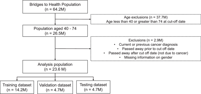
The population dataset from Bridges to Health (all those registered to a GP practice in England) is filtered to the age range of 40–74, and those with current and previous cancer diagnoses (relative to August 2021) are removed, resulting in an analysis dataset of 23.6M patients, which are then split into training, validation and testing datasets.
We use the period between August 2016 and August 2021 to construct our predictive features and patient histories. We then use these features to predict a cancer diagnosis in the period after September 2021. Our results focus on a 1-year predictive window between September 2021 and August 2022.
A stylised version of a patient pathway diagnosed with cancer in year 6 is presented in Fig. 2. In order to maintain a consistent length of 5 years of patient history, we used a single cut-off date for our analysis, and randomly split the analysis population between training, validation and testing. In the Supplementary Information (SI) we show results predicting up to 2 years after the cut-off date. We also present results when an exclusion gap is introduced after the cut-off date, to ignore diagnoses which may have occurred immediately after the cut-off date. These results are presented in the SI in the ‘Exclusion Gap’ analysis section.

The figure shows a stylised patient pathway with various types of events recorded during the 5 (history) + 1 (predictive window) years we observe the patients.
An individual’s patient history includes not only demographic information, but also comorbidities diagnosed during the 5-year period (between 2016 and 2021), as well as information on symptoms reported to NHS 111 lines. Individuals calling NHS 111 lines are triaged by trained personnel and based on their reported symptoms are referred to the appropriate services for further care. These could include primary care (with varying degrees of urgency), Accident & Emergency Care (A&E), or community/dental services. The dataset captures detailed information on the symptoms individuals reported as well as the type of referral (if any) the advisor made. For our analysis, we match the data on symptoms reported based on the pseudonymised patient number to the rest of the patient’s health record coming from their interactions with secondary care.
To create our patient histories, we complement data from NHS 111 lines with two national datasets. First, we use data from the Bridges to Health Segmentation (B2H). The dataset includes information on all individuals registered with a general practice in England and has rich information on demographics going beyond standard characteristics such as age, ethnicity and sex to also include household level information on the socioeconomic status of the household the person belongs to (e.g. urban professional). Household type information draws from the Acorn dataset23. The B2H itself draws from a large number of specialised national datasets covering health records beyond secondary care to also include mental health services and specialised tertiary care services. Drawing from this information several flags are created capturing a wide range of long-term conditions (e.g. COPD, physical disability, Downs syndrome). In our analysis, we only exclude those with the cancer flag as we want to ensure that our model predicts first incidence of cancer rather than recurrent cancer. In total, we include 59 binary features capturing a wider range of conditions from the B2H dataset. A detailed list of conditions is provided in Supplementary Table 1.
Second, we use data from the Secondary Uses Service (SUS) datasets and Emergency Care Services Dataset (ECDS) which covers all appointments/admissions and attendances to hospital secondary care services in England24,25. These datasets allow us to create features capturing the type of appointment the person had (e.g. outpatient appointment) and the associated diagnosis based on ICD–10 and SNOMED codes.
Data on mortality allows us to monitor who may have passed away after the cut-off date for reasons other than cancer and exclude those individuals from our data. We also exclude individuals with a previous cancer diagnosis. More details on dataset construction are included in the ‘methods’ section.
Note that excluding those passing away after the cut-off date due to other (than cancer) reasons could potentially introduce some bias in the results. However, the alternative is not without risks. Specifically, keeping those passing away from other reasons in our sample and treating them as negative cases (i.e. not diagnosed with cancer) would require assuming that none of the people passing away for other reasons (e.g. due to an accident) would have gone to develop cancer later during our prediction horizon. Clearly, a strong assumption which in our view could negate the potential advantages of including these individuals in our analysis.
Model prediction
We trained several classification models to predict the probability of being diagnosed with cancer in the coming year (September 2021–August 2022). We selected the XGBoost model as our preferred specification based on comparisons in terms of performance with the other classifiers (see comparison of machine learning algorithms in SI). Given the very sharp class imbalance between cancer and non-cancer cases, we use under sampling in our training datasets to ensure an equal number of cancer and non-cancer cases. We verified that the under sampled training dataset accurately represented the general control population on demographic variables such as age, gender, ethnicity and levels of deprivation (see Supplementary Table 7).
We predict the risk of cancer diagnosis for the nine cancer sites selected for the reasons discussed earlier. We also report the results for a model trained to predict any cancer diagnosis. By “any cancer diagnosis” we mean all cancer sites (see Supplementary Table 2 for ICD-10 codes) and not only the 9 cancer sites mentioned above.
For each of these models, we report several performance metrics for all cancer specific models, with a threshold value of 0.5 to ensure a balance between sensitivity and specificity (see Table 1). Each model was trained separately as a binary classifier. The ovarian cancer model was trained and tested only on females.
The size of datasets used for training, validation and testing for each of the cancer types is presented in Supplementary Table 3, and descriptive statistics on the whole population, and for the cancer and control population for each cancer site are presented in Supplementary Tables 4 and 5.
Important features
We demonstrate our approach for cohort construction by using bladder cancer, one of the priority cancer sites as our test case. In Table 2, we present some descriptive statistics focusing on the comparisons between those diagnosed with bladder cancer during the 1-year predictive window and those who were not.
As expected, there are noticeable differences in terms of age and gender between those diagnosed with bladder cancer in year 6 and those who were not. Cancer cases are predominantly male and older, reflecting the well-established link between age and cancer incidence, as well as the fact that bladder cancer is more frequent among males. Beyond demographics, the number of 111 calls reporting cancer related symptoms, as well as the number of A&E attendances, are higher on average for those diagnosed with bladder cancer in year 6 compared to those who are not. In total the model was trained on 821 features (see Supplementary Table 1 for full list).
Both the number of calls to NHS 111 lines reporting cancer related symptoms, as well as number of A&E attendances, will end up being among the most useful features for model prediction, as we will see later.
In order to improve model accuracy and to inform our work on constructing higher risk cohorts, we select the most important features using two metrics, gain and Shapley (SHAP) values.
In Fig. 3a, we show the SHAP values for the top 20 features (our models include 821 features in total) – ordered based on the gain metric (the average gain across all splits where the feature is used) for the XGBoost model (Fig. 3b). The red colour indicates higher values for the selected feature, and a positive SHAP value means an increase in the risk of cancer. For example, higher age has overwhelmingly positive SHAP values, which means that higher age is predicting higher risk of bladder cancer in the next year. By comparison, we show the mean absolute SHAP value for these features (Fig. 3c). While there are slight differences in the ordering of the most informative features, 17 out of the top 20 features based on average model gain are also amongst the top 20 features as determined by mean absolute SHAP value.

a SHAP value, shown by order of the top 20 features based on model gain value. Red (Blue) colour indicates high (low) values for the specific feature. Dots to the right (left) of the vertical line where SHAP value is zero indicate that this feature increases (decreases) predicted probability of cancer diagnosis in year 6. Features written in bold with an asterisk were also among the top 20 in feature importance based on mean absolute SHAP value. b XGBoost model average gain value c Mean absolute SHAP value for the top 20 features.
We observe that beyond age and gender, several comorbidities appear as relevant predictors of a bladder cancer diagnosis in ways that are consistent with expectations based on the medical literature. For example, the presence of chronic obstructive pulmonary disease (COPD) and urinary infections is associated with the incidence of bladder cancer in previous research26,27.
In addition, several features drawn from the NHS 111 calls dataset appear to be good predictors of bladder cancer incidence. For example, higher number of calls to NHS 111 lines reporting cancer related symptoms is one of the features with the highest gain metric value (just below demographics and long-term condition status). In addition, we also see that features capturing specific symptoms that are plausibly related to undiagnosed bladder cancer are also relevant and have the expected direction of effect. Specifically, higher number of calls to NHS 111 lines reporting “pain and frequency of passing urine” or “blood in urine” (during the last year) are both relevant predictors of risk of being diagnosed with bladder cancer in the next year.
To more comprehensively explore the importance of NHS 111 calls as predictors of risk of future cancer diagnosis, we replicated the analysis based on the gain metric for all other priority cancers beyond bladder. In all cases, features based on NHS 111 calls were among the most influential in predicting future cancer diagnosis. In Table 3, we report the rank of features, created from NHS 111 calls data, in terms of feature importance based on the gain metric. We do this for all cancer sites included in Table 1.
Table 3 highlights that features based on information captured in NHS 111 calls are among the top 20 features, based on the gain metric, and often among the top 5 or 10 for all cancer sites we explored in this study.
A comment regarding the predictive usefulness of symptoms reported in NHS 111 calls is warranted here. Some of the symptoms such as blood in urine may suggest that individuals would very quickly undergo medical evaluation which could lead to a relatively fast diagnosis of cancer. However, evidence from previous research on NHS 111 calls data suggests that a surprisingly high share of patients (close to one third) who are referred to urgent services such as emergency departments for a follow-up are actually not following the advice and neither appear to contact any other relevant health services following their call to NHS 11128. This means that it is very likely that many of the patients reporting what would appear as serious symptoms do not actually follow-up promptly thus postponing a potential diagnosis.
A possible concern with any analysis using patient histories is the possibility of data leakage. This could be the case if predictive features included in the analysis are indicative of a future cancer diagnosis in ways that undermine their predictive usefulness. For example, if a cancer diagnosis is recorded with a delay in the data, then it is conceivable that features strongly related with the diagnosis, such as cancer specific treatments, would “contaminate” the training data with the information about cancer diagnosis which we seek to predict. We however believe that this is unlikely to be the case here, for several reasons. First, our analysis excludes all those with a previous cancer diagnosis, and consequently also does not include treatments related to cancer as a predictive feature. Second, we do not include any cancer specific test results that could be construed as related to a future cancer diagnosis among our predictive features. Overall, the type of features we include such as demographics, symptoms reported in NHS 111 lines or comorbidities do seem much less likely to lead to such contamination as they are unlikely to be related to a yet not recorded diagnosis. Finally, we test our predictive models by excluding diagnoses in a time period after the cut-off date (see Exclusion Gap analysis in the SI) to confirm that our model can achieve good predictive performance even when focusing on cancers diagnosed more than 3 months after the cut-off date.
Constructing higher-risk cohorts
The primary goal for the analysis is to use the model results to construct high risk cohorts, for a cancer diagnosis within the next year, which can then be used to inform case finding and appropriate interventions to support earlier diagnosis and improve survival. We discuss two possible approaches to achieving this.
In the first, risk-based cohort construction method (Method A), we use the model risk probability at the individual patient level to create cohorts. Different sized cohorts can be constructed by varying the threshold for inclusion in the high-risk group.
The second feature-based cohort construction method (Method B) identifies cohorts with defined characteristics based on decision rules, utilising the most informative features from the trained model.
Method A: Risk based cohort construction
One approach to constructing higher risk cohorts is to consider capacity based on the requirements of a specific intervention/screening programme and then selecting the appropriate risk threshold which would lead to the desired cohort size. The risk thresholds are applied to the individual level predictions of the model. Based on different risk thresholds, higher risk cohorts of varying sizes can be constructed. The lower the risk threshold, the larger the size of the cohort, but the lower the potential incidence of cancer within the cohort. An illustration of this method is shown in Fig. 4.

Cohorts of different sizes are created by applying thresholds to model risk scores. The cancer incidence in such cohorts is calculated and compared to the baseline cancer rate to generate the lift value.
We define a lift value as the ratio of the cancer incidence within the cohort to the baseline cancer incidence. The baseline cancer incidence in our case, refers to those aged between 40–74 with no previous cancer diagnoses who go on to develop cancer in the next year. Based on different risk thresholds, one could construct a lift curve which plots the lift value against the size of the cohort on the x-axis.
An example based on the model on bladder cancer is provided in Fig. 5. The lift curve exhibits the expected shape where the lift value declines as we increase the size of the cohort. It also highlights the potential trade-off between high incidence and the total number of cancers correctly predicted. As the cohort size is increased, individuals with lower risk scores are included in the cohort, reducing the incidence and hence the lift value. The lift curve asymptotically approaches a lift value of 1—this represents the baseline cancer risk in the population (Fig. 5a).

Lift curve values for cohorts from a 0.5% to 100% of the population b 0.5% to 22% of the population. Predictions were obtained from a XGBoost model trained on all variables, and on another trained only on demographic variables to showcase the improved accuracy in identifying high risk groups when additional variables such as comorbidities and symptoms related to 111 calls are added.
Typically, the smaller the selected cohort of the population, the higher the lift value, as these are the individuals with the highest risk scores from the model. For example, in the top left of Fig. 5b, considering a cohort size of the highest risk (based on model probability risk score) 0.5% of the population (~125,000 individuals), the lift value of the model trained on all variables is 16, representing a cancer rate of 1 in 212 in the cohort. For a model trained on only demographic and socioeconomic variables (age, gender, ethnicity, IMD decile, integrated care board, acorn variables), the lift value for an equivalent cohort size is 9.4, representing a cancer rate of 1 in 357.
These values represent the potential order of magnitude improvement in cancer incidence in identifying high-risk cohorts using a risk score approach compared to chance selection from the population (cancer rate of 1 in 3355). If the cohort size is increased to the highest risk 5.8% of the population (~1.4 million individuals), the lift value reduces to 6.4 for the model with all variables (cancer rate 1 in 527) and 5.5 (cancer rate 1 in 613) for the model with demographic variables only. Lift curves for the other priority cancer sites are presented in Supplementary Fig. 4, and cohort cancer rates are presented in Supplementary Table 10.
These results also demonstrate the importance of including features from calls to NHS 111 lines, as well as comorbidities, to the model, as the resulting model risk scores can identify the highest risk individuals more accurately. As the cohort size increases, the difference in lift value between the two reduces, suggesting that both models capture the background demographic risk factors.
While more standard in terms of approach, Method A has several limitations from an operational perspective. First, Method A does not allow one to filter on features that may be most useful from a practical perspective. For example, depending on the type of intervention, one may want to focus on symptomatic patients and therefore select cohorts based on specific symptoms. Second, those charged with administering the interventions may not always have access to individual level predictions and instead would have to rely on flags drawing from specific features that are included in the data available to them. For example, eligibility for targeted lung health checks in England relies on age and smoking status.
This method also relies on applying thresholds to individual patient level predictions. While steps can be taken to explain the model (e.g. through feature importance and other techniques), ultimately the high-risk groups are a heterogeneous cohort. In Method B, we demonstrate how clearly defined cohorts can be created based on specific feature combinations.
A further limitation of this method is that the model may be biased towards predicting higher risk for certain demographic groups, making the high-risk cohort non representative of the actual incidence of bladder cancer in the population. As shown in the SHAP feature importance results (Fig. 3a), higher age, male, and white ethnicity all tend to increase the model risk score. This does correspond with higher incidence of bladder cancer in this group, however, given the low counts of bladder cancer among other demographic groups, it is difficult to ensure fair representation of all strata when constructing high-risk cohorts using this method, even when steps are taken to balance the training dataset. In the sub-group cohorts of Method B, we show how we sought to address this.
Method B: Feature based cohort construction
An alternative method that aims to overcome the above constraints is shown in Fig. 6 and outlined as follows. First, we select relevant features based on feature importance and data availability. The most important features, which were in the top 20 of model gain and SHAP value, were selected. SHAP was also used to identify the direction of the feature. Features which had a positive impact on the model output (i.e. which tended to increase the risk if the feature was present) were selected.

The most informative features from the trained model are identified and used to identify high-risk cohorts by identifying pairs of features which result in the cohorts with highest incidence. These decision rules can be applied either population wide, or to specific demographic sub-groups.
We then filter the population based on those features and examine the predicted cancer incidence. As is the case with Method A, we can then compare incidence of cancer in this curated cohort compared to the baseline incidence in the entire population.
This method has been applied to the whole population, and to sub-groups of demographic strata, demonstrating how the approach can be used for targeted interventions.
Population wide cohorts
The pair of features which would yield the highest incidence cohorts (on the validation data) of varying size (at least 10,000 to at least 250,000) were identified. Subsequently, the selected pair of features was applied to the test data to evaluate the expected bladder cancer incidence in the whole population. In Table 4, we show some examples of such curated cohorts based on combinations of just two features among those that the model considers as high importance for predicting cancer incidence in the next year. The cohort with highest cancer incidence, and a size of at least 10,000, is constructed based on interactions with the 111-call service and includes a specific bladder cancer related symptom of blood in urine. The cancer incidence within this cohort is 41 times higher than the overall incidence in the analysis population, with a cancer incidence of 1 in 82, compared to 1 in 3355 in the study population.
Larger cohorts of high-risk patients are constructed with flags relating to comorbidities of the genitourinary system and other diseases of the urinary system. Applying these flags to the population results in a cohort size of approximately 100,000 individuals, with a cancer rate 6 times higher than in the overall study population.
An example of a larger cohort of ~290,000 individuals would be constructed by applying the filter of patients having at least one long-term condition, and a diagnosis relating to symptoms and signs involving the genitourinary system in the last 5 years. This results in a cohort with a lift value of 4.5.
There is nothing in principle to prevent us from constructing cohorts based on combinations of more than two features (based on feature importance). Instead, our decision to opt for pairs of features is pragmatic. Especially when looking at population sub-groups based on gender/ethnicity (which we do in the next section) selecting more than two features would lead to very small cohorts, with sizes which are neither useful for practical purposes neither suitable for confidently inferring performance on the test dataset. As an example, the test dataset for the cohort of white males who had at least one call reporting cancer related symptoms in last year (AND) at least one call reporting blood in urine in last year (AND) have been diagnosed with hypertension includes just 517 individuals.
Sub-group cohorts
The population was segmented into demographic groups to investigate if different sets of features can create higher risk cohorts across demographic strata. This was also to address one of the limitations of method A, namely how we can ensure equality of opportunity if model predictions may be biased when there is insufficient training data from all demographic groups.
The segmentation was based on gender (male/female) and broad ethnicity (White/Non-white), resulting in four groups. Due to the low incidence of bladder cancer, more granular segmentation would have resulted in very small sample sizes.
For each population segment, the same methodology as described above was applied, with the cohort with the highest incidence of cancer cases being identified. These decision rules were then applied to the test dataset to evaluate the efficacy of the cohort. The lift value was calculated based on the incidence of cancer for each stratum. The results are shown in Table 5.
For the white ethnicity group, features related to 111 calls are particularly effective in identifying high risk groups. The specific nature of the symptom information (blood in urine) can result in small cohorts with lift values of 47.5 for white females, and 36 for white males.
In contrast, for the non-white ethnic group, more general health factors (e.g. A&E attendance) and comorbidities (e.g. COPD) result in the highest risk groups. These cohorts are still significantly higher in cancer incidence compared to baseline rates for these populations, as shown by the lift values of 2.9 for females, and 4.9 for males. However, they are also significantly lower than the lift values obtained for the white ethnic group. This potentially reflects health inequalities in the utilisation of services such as 111 calls. A key challenge here, which is not unique to our project, is the relatively fewer counts of cancer cases amongst the non-white ethnicities. For example, we observe only 97 instances of bladder cancer in the 1 year after the cut-off date in the non-white female population, compared to 4984 in the male white population. This presents the challenge of fewer samples to train the model on certain subgroups.
link